How heavy is your company’s loss tail? This question haunts every risk manager in one form or another, yet historical data rarely provides a definitive answer. A century of claims might contain only a handful of truly extreme losses, not nearly enough to distinguish between a tail shape parameter of 0.7 (catastrophic) versus 0.3 (manageable).
Traditional approaches either pick a single “best fit” tail shape (pretending we know more than we do) or run sensitivity analyses on a few discrete scenarios (missing the continuous nature of the uncertainty). What if we made tail uncertainty itself a first-class citizen in our simulations?
This article demonstrates a different approach: stochasticizing the parameters we’re most uncertain about, specifically the frequency multiplier and extreme loss tail shape, and exploring the full outcome space across insurance program designs. We use Sobol sequences (quasi-random sampling) to efficiently cover this high-dimensional uncertainty space, then analyze how nearly 25,000 insurance program configurations perform under 1,000 different tail scenarios.
The results reveal three surprising patterns about deductible and limit selection that only emerge when you explicitly model tail uncertainty.
Methodological Note: This analysis uses a simplified manufacturing company as a demonstration of the framework’s capabilities. The specific numerical results do not constitute insurance advice and should not be applied directly to real purchasing decisions. However, the methodological approach of stochasticizing uncertain parameters and using Sobol sequences for efficient exploration can be adapted to your specific situation. All corporate insurance purchasing decisions must be made in the full context of the individual company.
Company Configuration
I used the following company assumptions across all simulations:
- Initial Assets: $75M
- Asset Turnover Ratio: 1.0 (Revenue = Assets * Turnover)
- EBITA Before Claims and Insurance: 10%
- Tax Rate: 25%
- Retention Ratio: 70% (30% dividends)
- PP&E Ratio: 0% (meaning no depreciation expense)
Loss Configuration
The biggest changes in the configuration setup compared to prior analysis were making two parameters stochastic: a frequency multiplier, which scales the number of average losses experienced in a given year, as well as extreme loss tail shape, which influenced the tail thickness of very large losses.
These two parameters (frequency multiplier and loss tail shape) were scaled at the start of each configuration and held steady across all years and individual simulations.
Stochastic Frequency Multiplier
Real-world loss frequencies fluctuate due to changing operations, risk environments, and random variation. Rather than assuming a fixed Poisson mean, we make it stochastic by introducing a frequency multiplier that scales all loss frequencies proportionally.
The multiplier follows a Gamma(10, 0.1) distribution with mean = 1.0 and coefficient of variation ≈ 0.32. This creates scenarios where loss frequencies might run 30% below historical averages (multiplier ≈ 0.7) or 40% above (multiplier ≈ 1.4), while keeping most probability mass near the historical baseline.
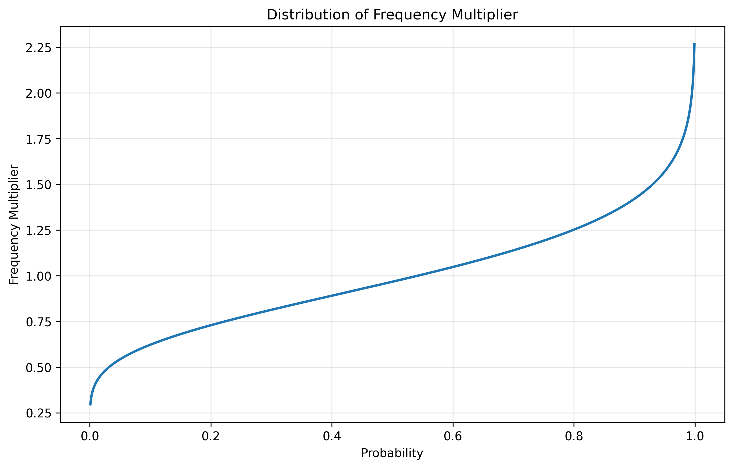
This single parameter scales all loss tiers simultaneously. If you experience more attritional losses in a given scenario, you also experience proportionally more catastrophic losses. While this simplifies away frequency correlation structures, it captures the intuition that risk environments have good years and bad years that affect all loss types.
Loss Distributions
The simulation employs a four-tier loss structure that captures the full spectrum from routine operational losses to catastrophic events:
Tier 1: Attritional Losses (routine operational incidents)
- Frequency: Poisson with mean = 21.38 × (Frequency Multiplier)
- Severity: Lognormal with mean = $40K, CV = 0.8
- Examples: Equipment damage, minor workplace injuries, small property claims
Tier 2: Large Losses (significant incidents)
- Frequency: Poisson with mean = 1.5 × (Frequency Multiplier)
- Severity: Lognormal with mean = $500K, CV = 1.5
- Examples: Major equipment failures, significant product recalls, material liability claims
Tier 3: Catastrophic Losses (severe events)
- Frequency: Poisson with mean = 0.15 × (Frequency Multiplier)
- Severity: Pareto with minimum = $5M, α = 2.5
- Examples: Facility fires, large product liability events, major supply chain disruptions
Tier 4: Extreme Losses (tail events beyond historical experience)
- Threshold: 99.95th percentile of overall loss distribution
- Severity: Generalized Pareto Distribution (GPD) calibrated to match catastrophic loss tail at the threshold, with stochastic shape parameter
- Examples: Company-threatening scenarios with limited historical precedent
Revenue serves as the exposure base, scaling all loss frequencies with company size. This structure assumes loss events are independent (no correlation), a simplification that understates systemic risk but allows us to isolate the effect of tail uncertainty on insurance program design.
Stochastic Tail Shape Parameter and Extreme Value Theory
When losses exceed a sufficiently high threshold, Extreme Value Theory (EVT) tells us that the exceedances follow a Generalized Pareto Distribution (GPD). This is a fundamental result in statistics, analogous to how the Central Limit Theorem justifies using normal distributions for averages. The GPD has two parameters:
- Scale (σ): Controls the overall magnitude of extreme losses
- Shape (ξ): Controls the tail thickness and fundamentally changes the distribution’s behavior
The shape parameter is critical for risk management:
- ξ < 0: Bounded tail (losses cannot exceed a maximum value)
- ξ = 0: Exponential tail (similar to normal distribution tails)
- ξ > 0: Heavy tail with infinite support (no theoretical upper limit)
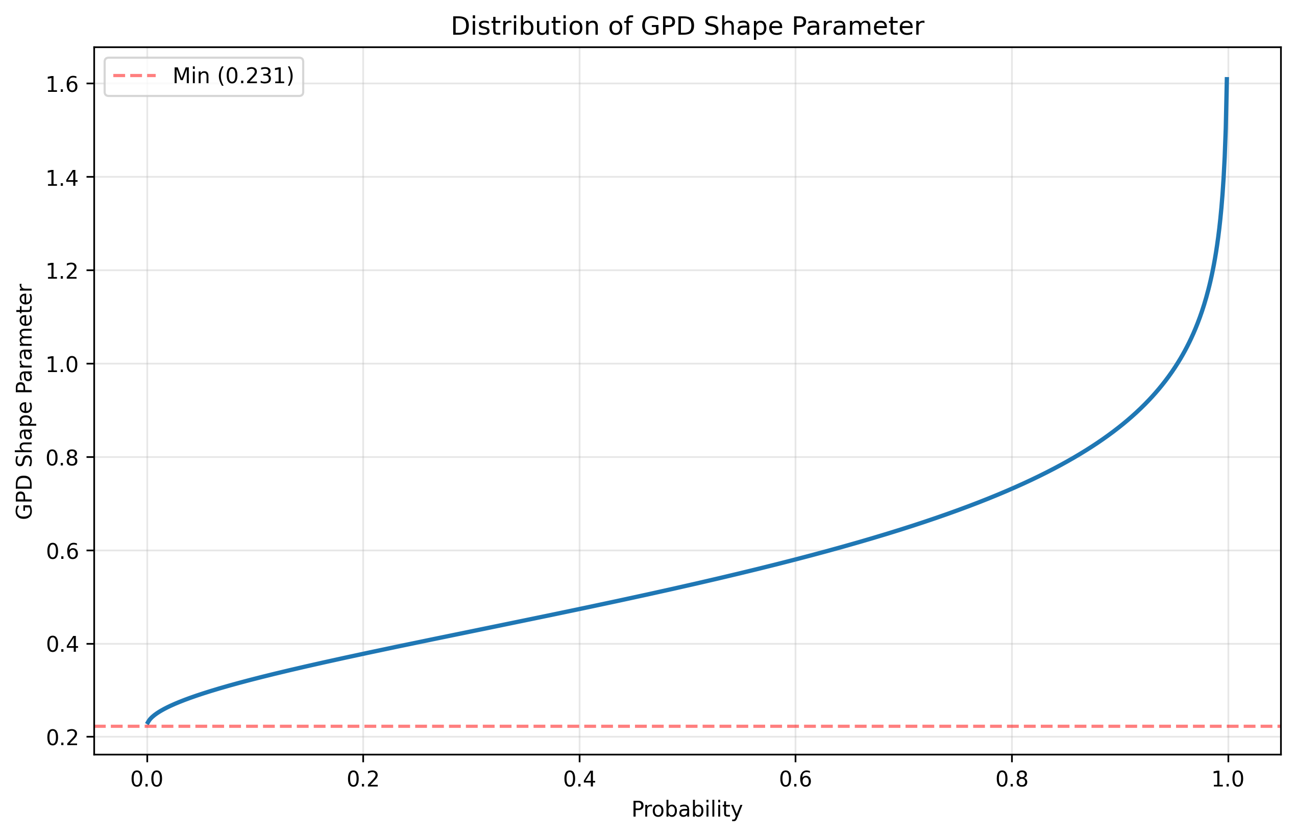
For corporate losses, theory suggests ξ typically falls between 0.2 and 0.8, but historical data is too sparse to pin this down precisely. This uncertainty is exactly what we’re exploring by making the tail shape stochastic.
In our simulation, the shape parameter ranges from approximately 0.23 to 1.5, with most probability mass between 0.5 and 0.8. Lower values produce thicker tails where extreme losses are both more likely and more severe. The distribution is constructed by starting with a Beta(2,3) prior, scaling it to [0.5, 0.8], then applying a logit transformation to allow for tail shapes outside this range while keeping most probability in the actuarially reasonable zone.
The GPD kicks in at the 99.95th percentile of our overall loss distribution (0.05% exceedance probability), replacing the Pareto-distributed catastrophic losses with the GPD to model truly extreme tail behavior. This threshold represents roughly 1-in-2000 loss events, or approximately one occurrence every 650 years given our base catastrophic frequency.
Sobol Sequences: Smarter Sampling for Tail Uncertainty
If you’re familiar with Monte Carlo simulation, you know the standard approach: generate random draws from your parameter distributions, run simulations for each draw, and average the results. With enough samples, the Law of Large Numbers guarantees convergence.
But “enough samples” can be prohibitively expensive when each simulation runs 10,000 paths over 25 years. More importantly, random sampling can miss critical regions of parameter space for hundreds or thousands of iterations by pure chance, which is particularly problematic when exploring tail scenarios that matter most for insurance decisions.
Sobol sequences offer a fundamentally different approach. Instead of random draws, they use carefully constructed quasi-random sequences that systematically fill multidimensional parameter space with maximum uniformity. Think of it as laying down a perfect grid that adapts to any dimensionality, ensuring proportional coverage of all parameter regions from the first sample.
Why This Matters for Tail Risk
In our 2D parameter space (frequency multiplier × tail shape), a standard Monte Carlo with 1,024 random draws might randomly cluster many samples in moderate scenarios (ξ ≈ 0.5-0.6) while leaving gaps in thin-tail regions (ξ < 0.3) or thick-tail regions (ξ > 0.8). Sobol sequences guarantee we explore thick, moderate, and thin tail scenarios in proportion to their probability from the start.
The practical impact:
- Faster convergence: Sobol-based simulations typically achieve comparable accuracy to pseudo-random Monte Carlo with 4-10x fewer parameter combinations
- Stable tail estimates: 95th percentile VaR and CTE metrics show much less sampling noise, critical when presenting results to leadership
- Reproducibility: Unlike random sampling, Sobol sequences are deterministic, meaning rerunning the analysis produces identical results
- Computational efficiency: We get production-quality insights with 1,024 Sobol points (2^10) instead of 10,000+ random parameter draws
For this analysis, Sobol sequences let us explore 24,576 insurance program configurations (1,024 parameter pairs × 4 deductibles × 6 limits) in 24 hours on Google Colab. The same coverage with random sampling would require 4-10x more parameter combinations to achieve comparable smoothness in the results surfaces you’ll see below.
Scenario Configuration
- Deductibles: $100K, $250K, $500K, $1M
- Policy Limits: $75M, $150M, $250M, $350M, $500M, $1B
- Loss Ratio: steady 60% across all configurations
This yielded 24,576 combinations of insurance programs and pairs of Sobol Sequence parameters.
For each configuration, I ran 10,000 simulations for 25 years. Although this is on the low side for production use, this setup ensured I could complete the runs in 24 hours on Google Colab and at a reasonable cost (less than $20 in CPU costs).
Key Assumptions & Limitations
This framework makes several simplifying assumptions that warrant discussion:
Insurance Market Assumptions:
- Uniform 60% loss ratio across all layers: Real-world pricing shows variation by attachment point—excess layers typically have much lower loss ratios (often 30-40%) due to higher pricing uncertainty, reduced competition, and larger insurer margins. This assumption understates the cost of high-limit programs (they’d cost roughly 1.5-2x more with realistic excess layer pricing), which is a limitation of this analysis. However, the ergodic penalty from a single uninsured extreme loss is so severe that high limits would likely remain advantageous even at significantly higher cost, though the optimal limit level might be lower than $1B.
- Perfect insurer knowledge: We assume insurers can price to the “true” loss distribution, including extreme tail scenarios. Reality involves information asymmetry and margin for uncertainty.
Loss Model Assumptions:
- Uncorrelated loss events: Loss occurrences are independent. This understates scenarios where multiple claims arise from a single event (e.g., supply chain disruption causing multiple customer claims). Directional insights hold, but absolute magnitudes would differ with correlated losses.
- Deterministic revenue growth: Revenue grows at a steady rate without volatility. Real companies face revenue uncertainty that correlates with loss exposure, which would amplify the value of insurance in economic downturns.
- No inflation or discounting: We ignore both premium inflation and the time value of money. Including these would modestly favor higher deductibles (invest the premium savings) but wouldn’t change the qualitative patterns.
Purpose and Limitations: These simplifications let us isolate how tail uncertainty affects insurance program selection without confounding factors. The specific numerical results (growth rates, optimal deductibles) don’t generalize to real companies. However, the qualitative insights that tail uncertainty makes limits more valuable, that median and tail scenarios can favor different deductibles, that thin tails neutralize deductible selection should transfer to more complex situations.
The framework can be adapted to include these complexities for company-specific analysis. Contact me if you need help with that.
Exploring Results: Three Surprising Patterns
With nearly 25,000 insurance program configurations spanning uncertain tail shapes and loss frequencies across 6.1 billion company-years, the results reveal three unexpected patterns that challenge conventional insurance wisdom.
Pattern 1: Buy Maximum Limits Regardless of Tail Uncertainty
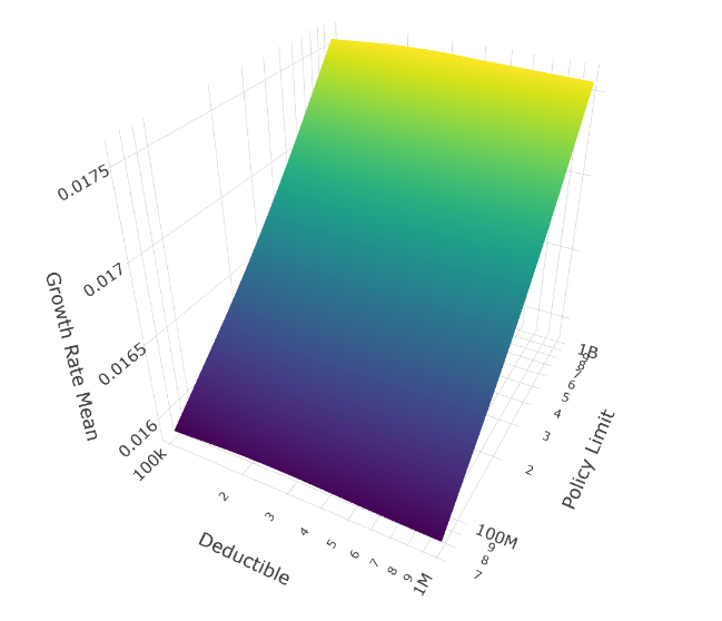
Across all deductible levels and tail scenarios, the message is unambiguous: higher policy limits consistently produce better time-average growth rates.
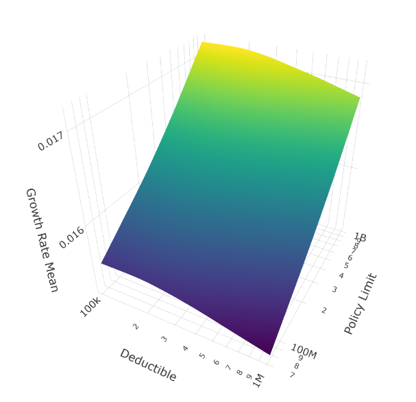 Mean growth rate across all 1,024 tail scenarios shows policy limits rising along the diagonal axis, deductibles along the horizontal. Higher limits (front-right) consistently deliver better outcomes.
The surface tilts decisively toward maximum coverage ($1B limits) regardless of deductible choice. This isn’t just risk aversion; it’s mathematically optimal for long-term compounded growth. When tail shapes are uncertain and can include very thick tails (ξ > 1), a single uninsured extreme loss can erase decades of premium savings from lower limits.
Why maximum limits dominate: With stochastic tail shapes, even a 5% probability of a thick-tailed scenario (where ξ > 0.8) creates substantial likelihood of losses exceeding $250M over 25 years. The ergodic growth rate penalizes sequences where one catastrophic loss destroys accumulated wealth, making high limits essential regardless of how rare such scenarios might be.
Pattern 2: The Deductible Paradox Where Median and Tail Preferences Diverge
If we look at median outcomes versus disaster scenarios, different deductibles emerge as optimal:
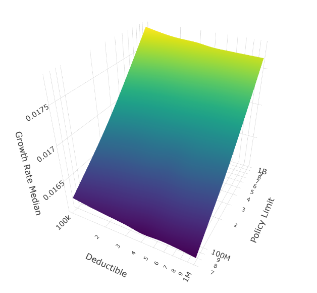
Median Growth Rate (Typical Scenarios)
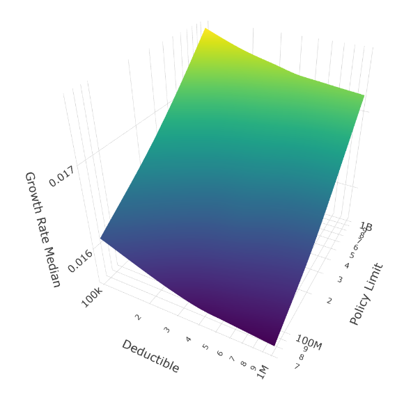 Median outcomes favor the $100K deductible for maximum insurance.
In the median scenario (50th percentile), the $100K deductible performs best. You might expect higher deductibles to win here through premium savings, but even in typical scenarios with our uncertain tails, enough large losses occur to justify maximum insurance.
5% Conditional Tail Expectation (Disaster Scenarios)
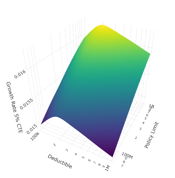 The 5% CTE reveals a different winner: the $250K deductible. Note the subtle but distinct depression at the $100K deductible position (left edge) compared to the $250K position (second from left).
But look at the worst 5% of scenarios (5% CTE), the very situations where you’d expect to want maximum insurance. The $250K deductible outperforms the $100K deductible in disaster scenarios.
This is counterintuitive but reveals a deep ergodic insight: In catastrophic scenarios, the compounding benefit of 25 years of lower premiums (from the higher deductible) outweighs the additional retained loss per event. When disasters strike, having preserved more capital through moderately higher deductibles provides more resilience than having paid for maximum first-dollar coverage.
The math: a $250K deductible might save $500K annually in premium compared to $100K deductible (at 60% loss ratio). Over 25 years of compounding growth through corporate reinvestment, that can be over $25M of additional capital. In thick-tail disaster scenarios, this capital buffer matters more than the incremental $150K of retained loss per catastrophic event.
Practical implication: For companies facing tail uncertainty, a moderate deductible ($250K-$500K range) combined with high limits may optimize both typical years and disaster resilience better than first-dollar coverage.
Pattern 3: Thin Tails Make Deductibles Irrelevant
Now filter to only scenarios with thin tails (ξ < 0.45), roughly the thinnest 30% of our tail shape distribution:
Mean Growth Rate (Thin Tails Only)
Median Growth Rate (Thin Tails Only)
5% CTE Growth Rate (Thin Tails Only)
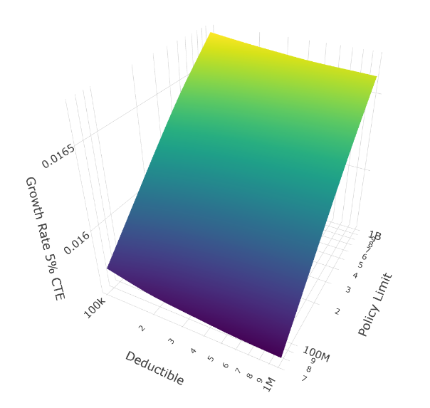
The surfaces flatten dramatically along the deductible axis. When tails are thin, deductible selection barely matters.
Why thin tails neutralize deductible choice:
With thin tails (ξ < 0.45), extreme losses decay rapidly. Looking at our loss severity structure:
- Attritional losses: $40K mean (far below any deductible)
- Large losses: $500K mean (comparable to mid-range deductibles)
- Catastrophic losses: $5M minimum with Pareto α=2.5
- Extreme losses: GPD with thin tail rarely produces mega-catastrophes
When the GPD shape parameter is high (thin tail), the probability of losses exceeding $50M drops by orders of magnitude compared to thick-tailed scenarios. Most losses land in the attritional and large loss categories, where:
- The $100K-$1M deductible range all respond similarly (either below the deductible or far above it)
- Premium differences from deductible choices shrink because expected retained losses are similar across deductible options
- Over 25 years, the compounding benefit of premium savings roughly equals the cost of retained losses
The limit dimension still matters even with thin tails, but only modestly. Notice the surfaces still tilt toward higher limits, just much more gently than in the thick-tail scenarios.
Practical implication: If you have strong evidence your loss distribution has thin tails (perhaps from extensive historical data), deductible selection becomes a secondary concern. Focus instead on ensuring adequate limits and optimizing premium costs through other program features.
The Meta-Insight: Sobol Sequences Reveal the Full Picture
None of these patterns would be visible with standard Monte Carlo sampling at our computational budget. The Sobol sequences ensured we explored thick-tail, medium-tail, and thin-tail scenarios proportionally from the first 1000 simulations, rather than potentially missing key tail regions until thousands of iterations.
Notice how the surface plots show smooth gradients rather than noisy artifacts. This is Sobol’s equidistribution at work. With pseudo-random sampling, we’d need 40,000-100,000 parameter combinations to achieve comparable coverage of the tail-shape × frequency-multiplier space.
Apply This to Your Company
The real power of this approach isn’t in these specific results; it’s in the methodology you can adapt to your own situation.
What parameters are you most uncertain about? For your company, it might not be tail shape. It could be:
- Frequency trends in a changing risk environment, such as in cyber, climate, supply chain (stochasticize Frequency)
- Correlation between different loss types during systemic events (stochasticize Frequency or Severity across layers)
- The effectiveness of new risk controls whose impact isn’t yet reflected in historical data (stochasticize Frequency or Severity of specific loss layers)
- Revenue volatility in emerging markets or new business lines (stochasticize the Asset Turnover Ratio)
The Sobol approach works whenever you can:
- Define a plausible probability distribution for uncertain parameters
- Evaluate insurance programs under each parameter combination
- Analyze how program performance varies across the uncertainty space
You don’t need 100,000 simulations to get useful insights. Sobol sequences with 1,024 parameter combinations (2^10) often suffice to reveal the patterns that matter for decision-making.
Getting Started
The complete implementation is available for you to modify and run:
Download the Code:
Install the Framework:
pip install ergodic-insuranceQuick Start Guide:
- Start with the example notebook to understand the structure
- Modify the company configuration to match your financials (lines 79-86 in the Python script)
- Adjust loss distributions to reflect your exposure (lines 98-102 for frequencies, 151-183 for severities)
- Define your uncertainty distributions for the parameters you want to stochasticize
- Run locally with smaller simulation counts (1,000 sims) or on Google Colab for full-scale runs
Need Help? The framework documentation includes:
- High-level overview and motivation
- Research paper with mathematical details
- Tutorial for adapting to your use case
A Challenge for Risk Managers
Next time you’re evaluating insurance programs, ask yourself: What parameter am I most uncertain about, and what would the decision landscape look like if I explicitly modeled that uncertainty?
You might discover, as we did here, that conventional wisdom (higher deductibles for worst-case scenarios, deductible selection matters most) doesn’t hold up when you properly account for tail uncertainty. The patterns that emerge from stochastic parameter analysis can fundamentally reshape how you think about risk transfer.
Try it on your own book of business. The insights might surprise you.
Next Application
- The Insurance Cliff When you plot the relationship between initial capital, policy limits, and bankruptcy risk, you don’t get a gentle slope. You get a cliff. In the active tail of modeled losses, where your business operates, the choice of limits has a disproportionate effect on results.